Internet use and income disparity: evidence from China

Data

CGSS, jointly administered by the National Survey Research Center (NSRC) at the Renmin University of China and a consortium of national academic institutions employs a stratified, multi-stage probability proportional to size (PPS) random sampling methodology. The survey comprehensively covers urban and rural households across all 31 provinces, autonomous regions, and municipalities in mainland China. Given its rigorous sampling framework and exhaustive geographic coverage, the CGSS data demonstrates strong national representativeness for socioeconomic research. There were 12,582 valid samples for the 2017 CGSS. The core independent variables for this study came from the Social Networks and Internet Society section of Module C in the total database. The section has a sample size of 4219. Those samples of this section were randomly selected from the CGSS sample map and are representative. This paper divides Internet use into access, usage ability, and usage outcome. The Internet access section includes users and non-users in the model. In this part, we removed samples with missing variable values, resulting in a final sample size of 4,144. Internet usage ability and usage outcome are further analyzed to determine how Internet use affects income disparity; therefore, we only use Internet access samples. The initial sample size for this section comprised 2377 observations. After excluding cases with missing variable values, the final sample size was 2299. It is important to highlight that the mean of the full sample was employed for imputation for cases with a limited number of variables containing outliers. We excluded cases with a substantial number of variable outliers.

Measurement of variables

Dependent variable

The dependent variable of this paper is income disparity. Referring to Kakwani’s research on “individual relative deprivation,” this paper employs the Kakwani index (Mantovani et al. 2020) to measure the income gap among Chinese residents. Within a specific group, the higher the income level of residents, the lower the relative deprivation they experience, the smaller the Kakwani index, and the lower the degree of income inequality. The calculation principle of the Kakwani index is as follows: Let Y represent a group with a sample size of n, and arrange the income levels of the group’s samples in ascending order to obtain the overall income distribution within the group: Y = (y₁, y₂, …, y_n). According to the definition, by comparing an individual with other reference individuals, the relative deprivation of the individual can be expressed as:

In Eq. (1): RD(y_j, y_i) represents the relative deprivation of y_j compared to y_i. Summing RD(y_j, y_i) over j and dividing by the mean income of the group, the following formula expresses an individual’s income inequality status:

In Eq. (2): \(\mu _Y\) is the average income of all surveyed samples in group Y, \(\mu _yi^+\) is the average income of surveyed samples in group Y with income exceeding y_i, and \(Y_yi^+\) is the percentage of samples in group Y with income exceeding y_i in the total sample size. The Kakwani index ranges from 0 to 1. The average income disparity for the whole sample is 0.614, with a maximum value of 1 and a minimum value of 0, indicating high-income disparity among Chinese residents. Among them, the average income disparity for the sample with Internet access is 0.515, and for the sample without Internet access is 0.747, showing a significant difference. It preliminarily suggests that Internet access has the effect of narrowing the income disparity.

Independent variables

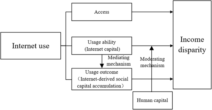
The core independent variable of this paper is Internet use, which is divided into Internet access, usage ability, and usage outcome. We use: “How often have you used the Internet in the past year?” to measure Internet access. The answer for this item is set to “daily,” “several times a week,” “several times a month,” “several times a year or less,” and “never.” If “never” is chosen for this question, assign a value of 0, indicating that there is no Internet access; choosing any of the other four options is assigned a value of 1, indicating access to the Internet. The results show that 57.36% of residents have access to the Internet.

Internet usage ability refers to the skills in utilizing and managing hardware and software equipment and obtaining, processing, and creating information on the Internet (DiMaggio and Hargittai 2001). By the definition above, this paper primarily examines four abilities: using the Internet to access social networking sites, downloading and installing smartphone apps, searching for desired information online, and expressing one’s thoughts through the Internet. The responses to the above items are scored on a scale of 1–5, with a higher value indicating stronger abilities. The KMO test result for the four items is 0.840, and Bartlett’s test of sphericity is less than 0.001, indicating that the four items are highly correlated and can be combined into one variable. We take the average of the four items as the value of Internet usage ability. Descriptive statistics show that the mean of Internet usage ability is 3.887, with a standard deviation of 1.138. The overall Internet usage ability of residents in China is relatively high, but there are also significant differences among different groups.

Mediating variable

Internet usage outcomes examine differential beneficiary patterns and capital accumulation mechanisms resulting from digital engagement (Deursen and Helsper 2015). Specifically, they capture the conversion outcome of Internet capital into traditional capital forms—economic, social, and human capital (Qiu et al. 2019). Given data constraints, this study focuses on Internet-derived social capital accumulation as the key usage outcome measure. Following Lin’s (2008) foundational work, we operationalized Internet-derived social capital accumulation through a network scale, measured by the survey item: “How many people do you contact daily via the Internet from Monday to Friday?” The ordinal response categories 1 = 0, 2 = 1–4, 3 = 5–9, 4 = 10–19, 5 = 20–49, and 6 = 50+ are treated as a continuous variable, where higher values indicate richer Internet-derived social capital accumulation. Descriptive statistics show that the mean of Internet-derived social capital accumulation is 3.111, with a standard deviation of 1.214.

Moderating variable

Human capital will moderate the impact of Internet usage ability on income disparity. We categorized human capital into two groups based on educational attainment: those with a high school diploma or lower and those with a college degree or higher. Descriptive statistics indicate that among the samples with a high school diploma or lower, 90% have not accessed the Internet, while 43% have. In contrast, among those with an associate degree or higher, 10% have not accessed the Internet, while 57% have. It is evident that human capital is positively correlated with Internet access; the higher the level of human capital, the greater the likelihood of accessing the Internet.

Control variables

Studies have shown that an individual’s age, gender, marital status, health status, household registration type, number of children, and region can affect income disparity, so we included them in the model as control variables. Table 1 shows descriptive statistics results for control variables.

Main models

The endogeneity issues between Internet access and income disparity include omitted variable problems, sample selection issues, and bidirectional causality problems. The Endogenous Switching Model (ESM) is a structural econometric approach capable of addressing multiple endogenous issues, particularly in settings characterized by self-selection bias and reverse causality (Yang 2021). Its key strength lies in explicitly modeling the selection process alongside outcome equations while permitting correlated error terms, thereby enabling more accurate causal inference (Christiansen and Peters 2020). (1) Self-selection bias. Individual choices may be influenced by unobserved factors (e.g., ability, motivation), biasing OLS estimates. The ESM estimates a selection equation (e.g., Probit/Logit) and computes the Inverse Mills Ratio (IMR) to control for selection bias. Moreover, ESM allows correlation between error terms of the selection and outcome equations (via Copula methods or joint maximum likelihood estimation), thereby correcting bias. (2) Reverse causality. Outcome variables may reciprocally influence selection variables, rendering OLS estimates inconsistent. The ESM employs a simultaneous equations model (SEM) to jointly estimate selection and outcome equations, circumventing unidirectional causality assumptions. (3) Sample selection bias. When observed data cover only specific subpopulations, estimates may be biased. The ESM extends the Heckman Selection Model to correct for such biases. Hence, we adopt ESM to examine the impact of Internet access on income disparity.

In addition, endogeneity issues also exist between Internet usage ability, usage outcomes, and income disparity. However, these two variables are continuous; the ESM is inapplicable, whereas the instrumental variable (IV) approach can effectively address omitted variable bias, measurement error, and reverse causality issues. Therefore, we tested the direct relationships between usage ability and income disparity using the IV approach. Moreover, causal mediation models examine the complex mechanisms linking Internet usage ability, usage outcomes, and income disparity. Given that other models are more conventional, the following sections primarily introduce the ESM.

Endogenous switching model. First, we adopted a probit model to estimate the Internet access decisions of individual i, expressing as Eqs. (3) and (4):

\(U_i^* \) denotes the potential reward difference between individual i accessing and not accessing the Internet. \(U_i\) is a dichotomous variable, \(U_i\) = 1 if the individual chooses to access the Internet; otherwise, \(U_i\) = 0. \(Z_i\) represents control and instrumental variables, including age, gender, education, marital status, health status, household registration, region, number of children, and instrumental variables. β is the parameter, and \(\mu _i\) is the error term.

The second step is the outcome equation, which divides the sample into two groups: Internet users and non-users.

\(Y_i1\) and \(Y_i0\) represent the income of individuals accessing and not accessing the Internet, respectively. \(X_i\) denotes the exogenous variables, i.e., the control variables listed above. \(\beta _i1\) and \(\beta _i0\) are parameters to be estimated, and \(\varepsilon _i1\) and \(\varepsilon _i0\) are random disturbance terms.

A selection bias may exist since \(\varepsilon _i1\), and \(\varepsilon _i0\) correlate with \(\mu _i\) in model 1. To resolve the bias, we can estimate selection Eqs. (5) and (6), calculating the Inverse Mills ratios (IMRs) \(\theta _i1\) and \(\theta _i0\). Then put \(\theta _i1\) and \(\theta _i0\) into outcome Eqs. (7) and (8).

Of which, σ_μ1 = cover (μ_i, ε_i1), σ_μ0 = cover (μ_i, ε_i0), IMRs \(\theta _i1=\frac\rm\varnothing (Z_i\hat\beta )\Phi (Z_i\hat\beta )\), \(\theta _i0=\frac\phi (Z_i\hat\beta )1-\Phi (Z_i\hat\beta )\), \(\gamma _i1\) and \(\gamma _i0\) are error terms.

The identification condition of the outcome equation is that at least one variable of the selection equation is different from the outcome equation. These variables influence whether to access the Internet but do not directly affect the individual’s income disparity, that is, instrumental variables. This paper draws on the research of Ma (2022) and Zhao and Li (2020), using the 2011 provincial Internet access rate (2011 PIA) and the distance from the individual’s provincial capital to Hangzhou (DPCH) as IV for Internet access. For 2011 PIA, on the one hand, the 2011 PIA may influence individuals’ opportunities for Internet access. On the other hand, it did not directly affect income disparity in 2017. Hangzhou is a core city of China’s Internet industry (hosting headquarters of major firms such as Alibaba and NetEase), boasts significantly superior Internet infrastructure (e.g., 5 G coverage, broadband speed) and policy support (e.g., the “First Digital Economy City” strategy) compared to other regions. Therefore, provincial capitals geographically closer to Hangzhou are more likely to benefit from spillover effects (e.g., technology diffusion, talent mobility, policy emulation) driven by Hangzhou’s Internet industry, thereby improving local Internet access levels. Moreover, historical and geographical factors determine DPCH and do not directly influence contemporary income disparity. Thus, both variables satisfy the relevance and exogeneity assumptions of IV. Based on the ESM framework, by comparing the income disparity of the Internet users and their expected value of the counterfactual outcome, we can calculate the average treatment effect of ATT and ATU (Khonje et al. 2015):

First, Eq. (9) expresses the actual income disparity of the observable Internet users in the sample.

If the user does not access the Internet, the counterfactual conditional expectation of his income disparity can be expressed as Eq. (10).

As a result, the ATT is the difference between Eqs. (9) and (10).

Second, Eq. (11) expresses the actual income disparity of the observable individuals in the sample who do not access the Internet.

Equation (10) expresses the counterfactual conditional expectation of their income disparity if non-users access the Internet.

As a result, the average treatment effect (ATU) is the difference between Eqs. (11) and (12).